Linear Regression is a very straightforward yet exciting algorithm. In my opinion, it is more of a statistical modeling algorithm than an actual ML algorithm. There is an excellent paper on the differences between statistical modeling and Machine Learning (algorithmic modeling) called Statistical Modeling: The Two Cultures which I would recommend to anyone interested in statistics and it’s relationship to ML. To summarize, Leo Breiman, the author of the paper, argues that the goal of statistical modeling is to try and simulate the relationships between the input data and the outputs while algorithmic modeling has a greater focus on the prediction of the outputs. This distinction is important because it gives the practitioner an idea of when it is suitable to use models such as Linear Regression and when it would be a bad idea. The algorithm has plenty of applications, including earning forecasting, credit loss forecasting, and even algorithmic trading.
What is Linear Regression?
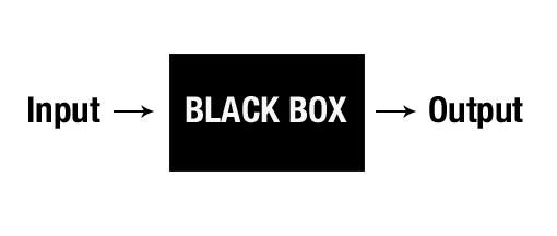
Linear regression is an example of a Supervised Learning algorithm where we use some input data and outputs to create a model that can predict outputs from new data. In any regression algorithm, our model has the goal of mapping the continuous inputs to outputs. Linear Regression does this mapping by creating a simple line that best ‘fits’ or generalizes the relationships between our input data and output data. This line can be best expressed by the equation y = mx + b. Where y are the outputs, m is the slope, and b is the y-intercept.
It might seem incredibly trivial to draw a line through some points. However, a computer does not have the same intuition as a human, and so we must come up with a computational way to do this. There are two main ways to draw this line, each with its benefits, Least Squared Error, and Gradient Descent. One may also use Mean Squared Error to implement Linear Regression, but it is usually more often used for checking the model’s performance. Regardless of what algorithm you decide to choose, it finds a line that has the shortest distance from the points.
How do we represent our data?
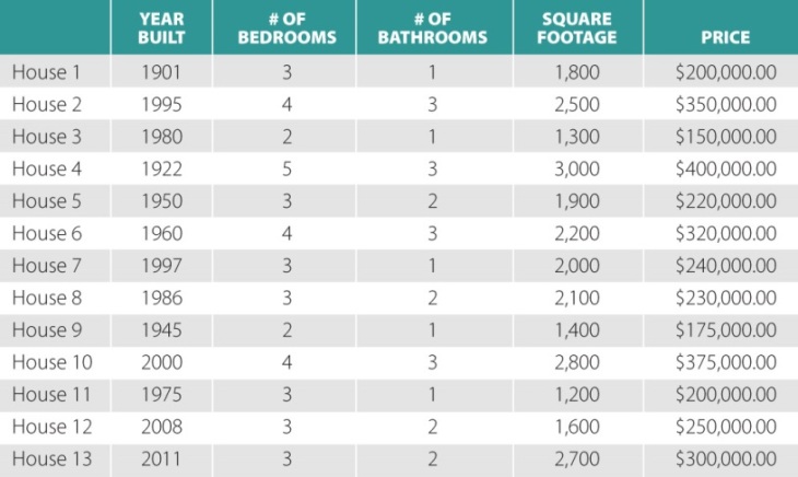
Before we begin talking about the algorithms themselves, let us establish how the algorithms view the data and how we can think about it intuitively. Let’s imagine that we only have one column of data or one feature as our input to best understand the concept. We represent our input data as X and our output/labels by y. Furthermore, we can represent our input and output data as matrices (when applying the algorithm we use NumPy arrays). We can also represent our y-intercept and slope as one matrix which we call the coefficient matrix. To do this, however, we need to add a column of ones to our input data because we want to obtain y = mx + b from every point.

As you can see our X(feature) and y(label) matrices are of size n by 2 and n by 1 respectively, where n is the number of data points we have in our dataset. We can further extend our matrix for multiple features by adding more columns to our feature matrix and making it size n by 1+k, where 1+k is the column of ones plus the number of features. The addition of columns to our feature matrix also means we need to add more rows to our coefficient matrix as shown below.

Polynomial Regression
This ability to modify the matrices is fascinating because it means we can also represent higher order polynomials instead of just linear functions by modifying the way we look at our matrices. Polynomial regression is incredibly similar to linear regression since in both we are trying to find the values for our coefficient matrix. I think it’s also important to mention that the higher the order of the polynomial the greater chance of overfitting. For example, if you only have 10 points in your data and you choose to have a polynomial of degree 10, then your best fit line is just going to go through all those points. This act of practically memorizing the data means that the model is not generalizing well enough and will most likely predict future values wrong. So how do you know when to use Linear Regression or a certain degree of Polynomial Regression? The simplest solution is to visualize your data and come up with multiple hypotheses that you can test out yourself.


Example Polynomial Regression
Least Square Error (Simple Linear Regression)
As stated above, we want to minimize the distance between the line and the points. In actuality, we want to minimize the sum of squared errors. The following equation obtains the sum of squared errors(where y are the label values given to the model, and y prime are the predicted values):

This equation is unique because it guides our model into obtaining the coefficients that give us the best fit line and is also used to measure the performance of our model. How we obtain the estimates from this equation is fascinating, and I recommend you check it out. The derived equations are as followed(where b_0 is our y-intercept, b_1 is our slope, X_i and Y_i our feature and label, and the X and Y with the line at the top are our mean/average values for the same feature and label):

The equation above gives us the coefficients that we need to create the line we’ve been trying to find. While the notation above is in a summation format, we can still try and translate it into matrix form which we’ll do in code. We will use a dataset obtained here which contains data for different body weights and their respective brain weights. We will treat our brain weights as a feature and our body weights as a label. It is also important to note that in python NumPy arrays are like arrays and will be used as matrices in this case. Therefore, our feature and label will be an array of 1 by n representing a matrix of n by 1. It does not have to be this way but for simplicity we will use this format.
import numpy as np
import matplotlib.pyplot as plt
X = np.loadtxt('new_file.txt', skiprows=0, usecols=(1))
y = np.loadtxt('new_file.txt', skiprows=0, usecols=(2))

def find_coef(X, y):
    #calculate the mean values
    X_mean = np.mean(X)
    y_mean = np.mean(y)

    #use the formula to calculate the values
    slope = np.sum((X-X_mean)*(y-y_mean))/np.sum((X-X_mean)**2)
    y_intercept = y_mean-slope*X_mean
    return(slope, y_intercept)

plt.scatter(X, y, color = "m", marker = "o", s = 30)
(m, y) = find_coef(X, y)
y_pred = y + m*X
plt.plot(X, y_pred, color = "g")
plt.xlabel('Brain Weight')
plt.ylabel('Body Weight')

It is interesting to see that we can implement a summation as matrix or array operations. NumPy provides a very efficient and simple way to do this and I recommend looking at more of NumPy’s features before continuing on your ML journey. Regardless, as you can see the brain weight increases as the body weight increases and we can conclude that they have a positive correlation. The coefficients that our algorithm generated are
slope = 1.2284714375404622, y-intercept = 36.57230942629311
What about more Features?
Something is off. You might have noticed that we didn’t correctly use the matrix format described previously. We decided to use a 1 by n array instead of an by 1 array, and we didn’t add the one’s column! The above implementation wouldn’t work for multiple features and would especially not work for polynomial regression. For this, we are going to use a more complex equation known as the Normal Equation which can be derived from Least Squares or Mean Squared Error using their gradient. The theory behind this is incredibly long, so I am only going to show you the equation and our implementation of it. You can learn more about it here.

def find_coef(X, y):
    #calculate the amount of data points
    points_count = np.size(X)
    #reshape our features array into a n by 1 array/matrix
    #also add the column of ones
    X = np.hstack((np.ones(points_count).reshape((-1, 1)), X.reshape(-1,1)))
    #normal equation
    coefficients = np.linalg.inv(X.T.dot(X)).dot(X.T).dot(y)
    return coefficients
The code abode will return an array of coefficients which will correspond to their own feature and the y-intercept. This means that we can use more than just one feature in order to predict our label. This is great news! I am not going to bother showing the graph again because it is exactly the same. Finally, the coefficients return for this implementation are very much the same as the simple linear regression implementation:
slope = 1.22847144, y-intercept = 36.57230943
Gradient Descent
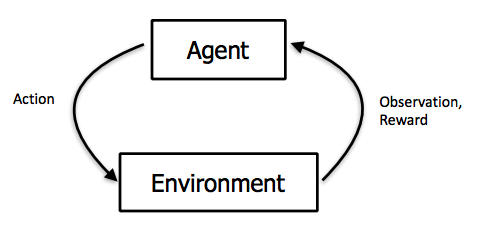
The algorithm is widely used in Machine Learning and is especially powerful when used in Deep Neural Networks and the backpropagation method. I’ll cover the math behind Gradient Descent in a future blog post. For now, let’s look at the bigger picture and how it works in Linear Regression.
The computer starts calculating the best line by first drawing a random line. This means that it has random values for m(slope) and b(y-intercept) in the equation y = mx + b. It then calculates the error by calculating the distance between the points and the line(same concept as before). Gradient Descent then tries different lines to reduce the error. If the algorithm notices that the error decreases then the line moves in that direction. If the error increases then we move in the opposite direction.

This simple process is very powerful and is actually the preferred method for linear regression in many libraries. It is way more efficient then the implementations above. This is especially true when dealing with more features and when dealing with higher order polynomials.
Resources
- Scikit-Learn Linear Regression (We didn’t cover scikit-learn because they already have easy to understand examples)
- MIT 6.S085 Linear Regression Notes